Flight Delay Predictor

By Stan Huang and Xiaosong Yin

EECS 349 Machine Learning
Northwestern University
Advised by: Doug Downey

Contact:
stanhuang2017@u.northwestern.edu
xiaosongyin2017@u.northwestern.edu

---

Table of Contents 

Introduction
Overview
Our Goal
Data
Results
Analysis
Conclusion
Future Steps

Introduction

Over 700 million people in the United States travel by air. Flying has become routine for many people who greatly value their time, and as travelers increasingly rely on airline companies for reasonable on-time performance, many of them fear departure delays that might ruin scheduled appointments or plans. While weather delays can be easily predicted by the severity of the weather, many passengers buy tickets long before any weather data is even up, but would still benefit from being able to predict a delay based on other telling factors.  Planes still suffer delays due to the overall efficiency of the plane preparation process, which is most likely dependent on the carrier, airports, and number of passengers a flight will have.

With this in mind, we decided to create a tool that can predict the expected delay status of domestic flights based on historical flight data.  Our program will use conditions such as origin, destination, number of passengers, carrier, and delay times/reasons in order to learn whether a plane will be delayed. The tool will allow users to input an origin, destination, carrier, and in return will receive a delay prediction on a). how likely is the flight going to be delayed and b). by how much time will the flight be delayed.

Overview

Our data size will be over a million, but we will work with 100,000 of the entire data set. In our tests, we will follow two different ideas and see which one yields a better result. We will run KNN for one of the tests and J48 decision tree for the other one. In our analysis section, we will talk more about each one and their performance.

Our Goal

As a team we worked together to set goals for our project. We decided before starting the project that our project must be reasonably quick. We are assuming that anyone who wants to predict a delay would prefer not to waste too much time waiting for the results. The second goal we set ourselves was to get ensure that we could reach at least 75% in our project’s accuracy. We decided that the lowest performance we would allow is accurately predicting three out of four flight delays statuses.

Data

We collected all data from on-time domestic flight information provided by the Bureau of Transportation Statistics located at http://www.rita.dot.gov/bts. From this data we extracted the following attributes:

• Month
• Depature Time: in hhmm format, local time
• Arrival Time: in hhmm format, local time
• Air Carrier: identified by a unique air carrier code (AA for American Airlines, etc.)
• Origin Airport: identified by a unique airport code
• Destination Airport: identified by a unique airport code
• Air Time: the duration of a flight in air
• Distance: distance between airport
• Origin Airport State: identified by the state code
• Destination Airport State: identified by the state code
• Arrival Delay Time: number of minutes delayed upon arrival
• Carrier Delay: this is the information we are trying to predict.

From this data we used MATLAB to do some pre-processing and partitioning in order to make the data a little easier to work with. First we cut down on the amount of data we had. When we had finished collecting data, we had nearly a million data points, so we wrote a script to create a new csv containing every 60th iterated data point to bring us down to a more workable 100,000 instances.

A sample of the original data is shown in the table below:

MONTH	CARRIER	ORIGIN_AIRPORT_ID	DEST_AIRPORT_ID	DEP_TIME	ARR_TIME	AIR_TIME	DISTANCE	ARR_DELAY	CARRIER_DELAY
1	9E	10397	10423	1425	1553	118	813	203
1	9E	10397	10423	1228	1356	118	813	86
1	9E	10397	10423	1053	1230	128	813	0
1	9E	10397	10423	1047	1226	135	813	-4
1	9E	10397	14492	1753	1918	54	356	-2
1	9E	10397	14492	1755	1915	56	356	-5
1	9E	10397	14492	1846	2017	51	356	57
1	9E	10397	14492	1859	2012	51	356	52
1	9E	10397	14492	1752	1918	61	356	-2

Analysis

We decided to use MATLAB primarily for data processing and WEKA for running different algorithms on the dataset. Further, we originally proposed two strategies to tackle this problem. Each strategy leads us in a different direction as to how we do the data processing process.

The first strategy is the “keep-data” strategy. We keep all the fields as they are in its original shape. In this strategy, we run Nearest Neighbor related algorithm.

The second strategy is the “partition” strategy. In this strategy, we partition each field into a limited number of categories so that decision-tree related algorithms are more suitable in this case. . Below is the method we used to partition the data:

• Departure Time: partitioned into morning, afternoon, evening and late night
• Arrival Time: similar to departure time
• Air Carrier: partitioned by number of appearances in the dataset. More appearance equals larger carriers
• Origin Airport: partitioned by number of appearances
• Destination Airport: similar to origin airport
• Air Time: partitioned by number of hours
• Distance: partitioned by 100 miles
• Origin Airport State: partitioned into regions – Northeast, Northwest, South, West, Pacific, and Other. This was done manually through the dataset using excel

How we used the partitioned data and the rationale are explained in detail in the report.

For both of the two strategies, we ran two different sets of tests. All tests are performed under the 10-fold validation setting except for some instances of KNN where we did split train/test for the sake of speed.

1. Whether the flight is delayed or not. In this case, we set a new field called “delay” to 0 or 1 based on the arrival delay attribute. Here, we also need to make a decision to define delay. We tried three strategies for comparison. In this first one, a flight is not delayed if the arrival delay time is below or equal to 0 (if you arrive 1 minute late, you are delayed). Second, a flight is not delayed if it arrives 5 minutes or less late (if you arrive 6 minutes late, you are delayed). Third, a flight is not delayed if it arrives 10 minutes or less late (if you arrive 11 minutes late, you are delayed).
2. How much is the flight delay. Here, we set three scales: less than 30 minutes, less than 120 minutes and more than 120 minutes. We decided that passengers are most concerned about the half-hour and two-hour threshold regarding a delay.

All our MATLAB scripts can be found on our git repository:
https://github.com/shuang2831/Flight-Delay-Predictor

Results

We have two sets of analysis corresponding to our two different strategies.

In the “keep-data” strategy, we tried different number of attributes to put into the test and different settings on the Ikb algorithm built into WEKA (used 1-NN and 5-NN). The average accuracy is ~71%. In more detailed analysis:

• The algorithm works better if we don’t have “Arrival Time” and “Departure Time” as attributes. The result is 73% if we don’t have them and 68% if we do.
• The 5-NN setting performs slightly better than the 1-NN setting with a 1% difference.
• The algorithm trains very slowly on the dataset

Although there seems to be a correlation among similar flights, the accuracy level does not meet our goal.

In the “partition” strategy, we used J48 tree built into WEKA. We varied a few parameters on the tree (turned on/off error-reduced-pruning). The average accuracy is ~75% with the correct set of decision-making on the dataset. In more detailed analysis:

• Reduced-error-pruning increases the accuracy in some cases and decreases the accuracy in others.
• It trains the dataset much faster than KNN.
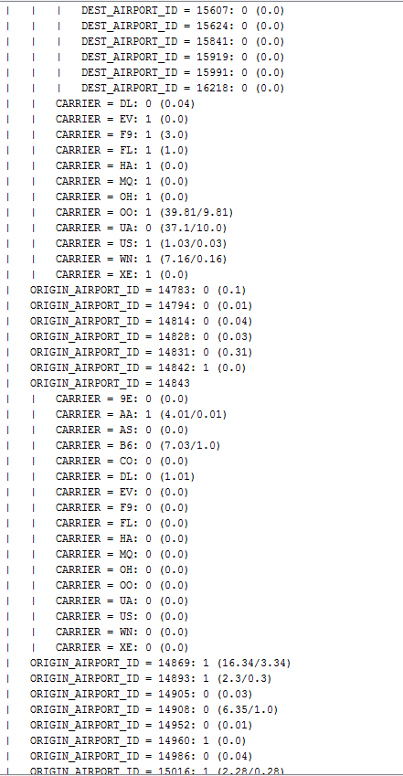
• The most information gain comes from departure / arrival time since they end up in the root of the decision tree
• Also valuable is the original airport. The detailed list of attributes as they stand in the decision tree is shown below
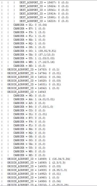
• As one can see from the list, following original airport is carrier, after that is destination airport.

The two most important decisions about the dataset in this case are how we define delay and what attributes we include for the test. The results with each setup is summarized in the table below with each row being 0, 5 or 10 minutes for defining delay (please see the previous section for the definition) and each column being attribute inclusion.

Delay definition / Attribute Inclusion	No Departure / Arrival Time	Departure / Arrival Time
>0 minutes	65%	—
>5 minutes	68%	73%
>10 minutes	73%	78%

As one can see from the table, since departure time / arrival time are the most importance pieces of data, they increase the accuracy of the model by ~5%. In addition, by setting the delay definition to 10 minutes, we have a lot better accuracy in telling whether a flight is delayed or not.

The best accuracy we can achieve by this strategy is 78%. This meets our goal.

A snapshot of the WEKA result page for the accuracy is shown below

Below is a cross-method comparison between KNN and J48 decision tree for different setups we had. From this graph, one can see that our delay definition has little impact on KNN but large impact on J48. Both data are positively impacted by the inclusion of the additional arrival / departure data.

When we run the previous tests to predict which delay level a flight is likely to fall, the accuracy drops to as low as 54%. Recall that we divided the delay level to =120 min.

There are a few reasons for such a low accuracy. Compared to the binary prediction of whether a flight is delayed or not, there are much fewer instances where flights are delayed for longer time. Thus, the data set is magnitude smaller than the original. Also, when a flight is delayed for longer time, it is more out of random possibility (aircraft suddenly needs maintenance, the previous aircraft arrives late, etc.) so that there is far smaller correlation between such cases with the data we collected. Due to these factors, our model proves little use to predict how long a flight is likely to delay.

Conclusion

Our model predicts whether the flight or not at an accuracy of 78%, meeting our preset goal and provides a reasonable reference for the user. Our model, however, does not perform well when predicting how long a flight is likely to be delayed.

In our analysis, we took two alternative approaches to tackle the problem, one of them keeping the data set in the original form while the other one partitioning data into more general forms. The latter proves to be the better choice while the former is also acceptable despite below our standard. From the results, we can see that there is indeed some degree of correlation between the data and the likelihood of delay. The most telling attributes towards delay or not are departure / arrival time and departure / arrival time.

Future Steps

While we found the J48 decision tree to be the best classifier to use for the data that we partitioned and used, we believe that there are possibly methods that would work even better since 78% barely passes our basic goal.

Another step we’d love to take is finding more complex ways of manipulating our data to fit the needs of the classifiers. We partitioned most attributes into different rankings and categories, but we believe more could have been done. If we had the chance we would dive into designing various algorithms that would alter the data in different ways.

One last step would be to be able to run the project on larger sets of data over various years. The amount time span of data we used was very limited having around only 2 or 3 years of data to learn from. If possible we’d like to find a way to download at least a decade of date and efficiently pick out enough instances to have our project learn from.

Link to full report:

Flight Delay Predictor Full Report